Jul 23, 2025 33 min read Stata

Do we need to use cluster variance in Difference in Difference models? Revisiting an old paper

In 2002 Bertrand, Duflo and Mullainathan published an influential paper at the National Bureau of Economic Research (NBER) which argued that difference-in-difference studies have a fundamental problem of under-estimating variance, and proposed some solutions to this problem. In this paper they argued that the estimates from two-way fixed effect (TWFE) regression designs for difference-in-difference (DiD) studies have standard errors that are too small, and suggested that this was due to auto-correlation that is induced by the research design, in particular the difference-in-difference term in the regression model. They argued that this was an inescapable consequence of the fixed effects in the model, and suggested four different methods for solving this problem. Since the publication of this paper, clustering the variance estimates became the preferred solution to this "problem", and is commonly done in almost every analysis conducted by econometricians using TWFE models.

I think there are some serious problems with this paper, and that it has led econometricians down a bad path by suggesting a solution (clustered variance) to a model type (TWFE) that is fundamentally flawed. In this post I will discuss the problems with the original paper, present a simpler, improved simulation that shows there is no "problem", and argue that researchers do not need to cluster variance in difference-in-difference regressions.

The code for this post is available in a Github repository.

Introducing the paper

The original paper, hereafter referred to as BDM2002, can be viewed at the National Bureau of Economic Research webpage here(pdf!). The structure of the paper is as follows:

The authors introduce the fundamental TWFE model structure
The authors conduct a quick, unsystematic review of published papers to show the kind of studies that have been conducted using TWFE models
They conduct a simulation study using data from the Current Population Survey (CPS), in which they run a series of fake interventions on the data, and show that even though there should be no "true" intervention effect, simple TWFE models find a highly significant intervention effect
Using some analysis of this regression structure, they argue that this under-estimation of standard errors is due to auto-correlation(1)
They suggest several solutions to the problem, some of which are disastrous and some of which are complicated and potentially computationally intensive

We will test this data later in this post. Before we examine their approach, however, let's look at the TWFE model they use. They suppose that they have a set of data with $T$ time points, $S$ observation groups (e.g. states) and $n_S$ individuals in each group. These are indexed with:
$i=1,\ldots,n_S$,
$s=1,\ldots,S$,
$t=1,\ldots,T$,

We have a response $Y_{ist}$, fixed effects $A_s$ for state and $B_t$ for time, and a TWFE difference-in-difference term $T_{st}$, coded such that

$ T_{st}=1 $ if the observation is in the treatment group in the treatment period
$ T_{st}=0 $ otherwise

So, for example, if we have $S=10$, and the treatment begins at time point 6, then $T_{st}$ will be 1 for states that are in the treatment group after time $t=6$, it will be 0 for states in the treatment group before time $t=6$, and 0 for states in the control group at all time points.

We can also assume we have a matrix of covariates, $X_{ist}$ and a corresponding vector of coefficients $c$. Then we construct the OLS regression equation for a TWFE model as:

$$ Y_{ist}=A_s+B_t+cX_{ist}+\beta T_{st}+\epsilon_{ist} \tag{1}$$

The difference-in-difference model estimate of the treatment effect is $\beta$, and we assume the residuals $\epsilon_{ist}$ are normally distributed with mean 0. In a classical OLS regression it is assumed that the residuals in equation (1) are independent and identically distributed. There are no correlations between individuals within or between states or within or between time points.

I have a lot of issues with this model design, arising primarily from the fact that the treatment term $T_{ist}$ is actually a second-order interaction term, but its main effects are not included in the model. These issues are not relevant to this post, however, which will restrict itself to the variance-clustering issue, so let's discuss some problems with this article on the assumption that TWFE is fine to use.

Problems with this paper

There are three key problems with this article, which I think undermine its central thesis. These are:

It "simulates" its models using real-world data from the CPS, rather than properly simulated data, so we don't know the truth of the underlying model and cannot conclude whether the simulation is showing a fact about the data or a flaw in the model
The investigation of auto-correlation and its proposal as an explanation is weak
The results of the simulation model are not presented in detail, so it's difficult to say how serious the "problem" of models rejecting the null hypothesis actually is. With a very large data set it is possible to have situations where non-significant variables become significant by dint of the sheer size of the data, and we need to examine the overall structure of the model to properly understand the meaning of spurious signifance

The first two problems are at the core of the issue with this paper, so let's investigate them first.

Problems with using real world data for simulation

This article uses data from the CPS to test whether TWFE models under-estimate standard errors. Here is their description of the data they obtain from the CPS:

We extract data on women in their fourth interview month in the Merged Outgoing Rotation Group of the CPS for the years 1979 to 1999. We focus on all women between 25 and 50 years old. We extract information on weekly earnings, employment status, education, age, and state of residence. The sample contains nearly 900,000 observations. We define wage as log(weekly earnings). Of the 900,000 women in the original sample, approximately 300,000 report strictly positive weekly earnings. This generates ($50*21=1050$) state-year cells with each cell containing on average a little less than 300 women with positive weekly earnings

In the simulation chapter, they describe the simulation process as follows:

To quantify the bias induced by serial correlation in the DD context, we randomly generate laws, which affect some states and not others. We first draw at random from a uniform distribution between 1985 and 1995. Second, we select exactly half the states (25) at random and designate them as “affected” by the law (even though the law does not actually have an effect). The intervention variable Tst is then defined as a dummy variable which equals 1 for all women that live in an affected state after the intervention date, and 0 otherwise. We can then estimate DD (equation 1) using OLS on these placebo laws. The estimation generates an estimate of the laws’ “effect” and a corresponding standard error. To understand how well DD performs we can repeat this exercise a large number of times, each time drawing new laws at random. If DD provides an appropriate estimate for the standard error, we would expect that we reject the null hypothesis of no effect (β = 0) exactly 5% of the time when we use a threshold of 1.96 for the t-statistic

The theory here is that, since there is no intervention in any of the years between 1985 and 1995, there is no reason to suppose that a randomly generated sub-sample of states with a randomly generated intervention period in this 10 year period would be associated with a significant effect, so if we find lots of significant terms in these randomly simulated null interventions, we should conclude our modeling process is wrong.

The problem with this is that we don't know what is true about this data. Between 1979 and 1999 there were huge changes in the rights of women at work, and a steadily declining gap between women's and men's wages. There was also a recession in 1990, during which GDP shrank by 1.4%. It's possible therefore that the trend in women's wages was not linear, and in a short time series like this (just 10 years of data) it's very possible that a small step or curvature in wages, if not properly handled by the basic structure of the model, will be picked up by the intervention term. Furthermore, over the period of the study more women entered work (which might drive wages down), but the population aged (which typically drives wages up) and women were less likely to drop out of work due to childbirth (which would change the structure of the wage data). It's difficult to say how this would be reflected in the data, and since we don't know the "truth" about this data and its underlying structure, we cannot authoritatively conclude that the findings of any particular statistical model are wrong.

We can test this by downloading the data and examining it. BDM2002 do not provide their code or data, but I found a random Stack Overflow post by someone who was reproducing their results, and was able to download and prepare the data basically as it was used in the paper. The Stata do file bdmPrep.do performs this download, and also plots some basic data. There is a huge amount of data, so if we plot the entire data set we don't see anything meaningful, but we can select a single year of age and a state to plot, and see what the data looks like. Figure 1 shows some data for different ages and states, that I picked arbitrarily.

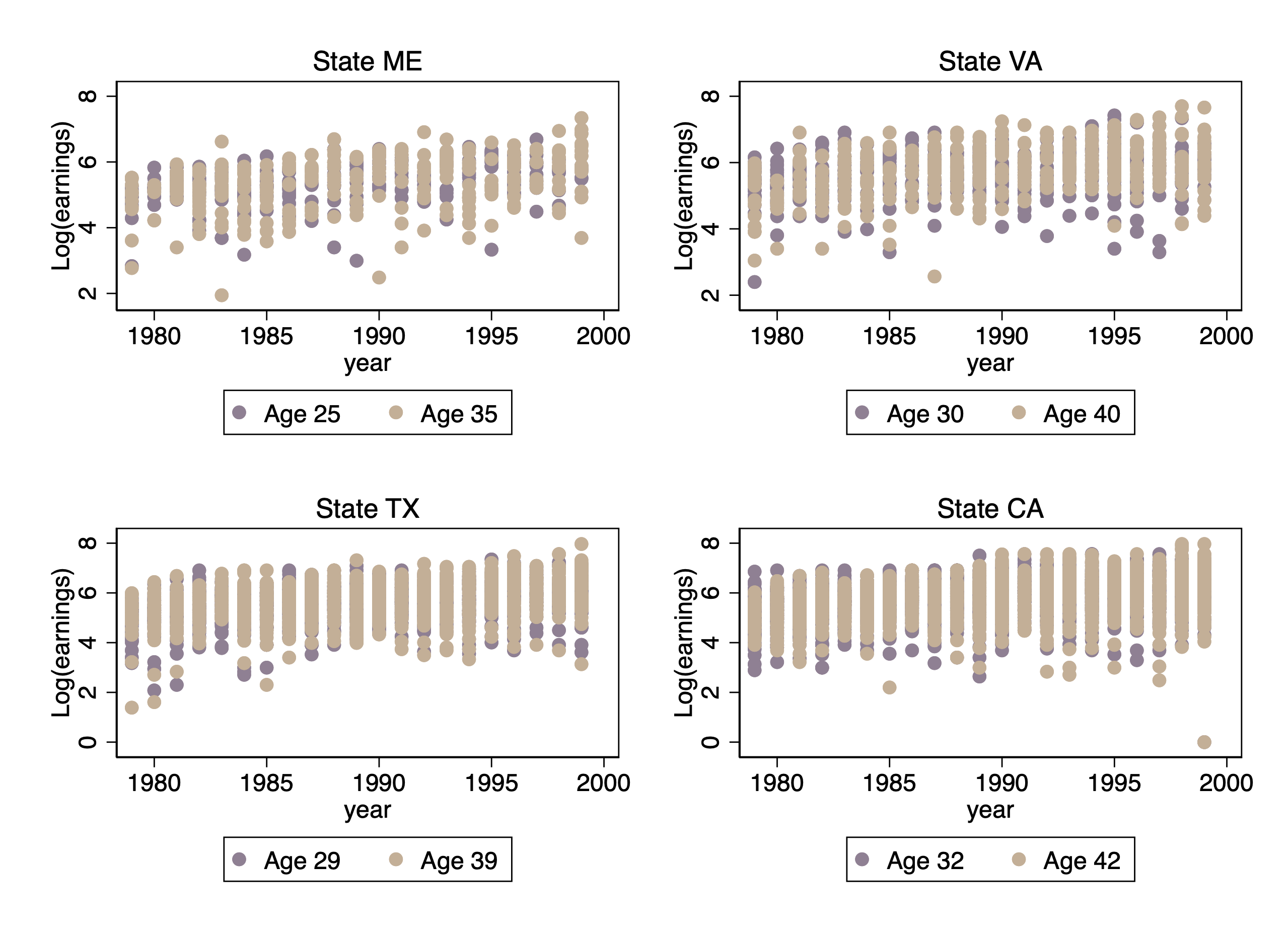
Figure 1: Log earnings by year for four arbitrary states and age groups

It appears that there is a slight trend in the data, and also some changes in extrema: in the state of ME, for example, the minimum values go from 2 in 1979 to about 3.5 in 199; we see similar patterns in VA and TX. There seems to be a weird outlier in California (CA), but also there are so many data points it's hard to see a pattern except that the data may be rising.

We can conduct a simple linear regression without considering any DiD model, and examine the trends and patterns in wages from that regression. For example, if we build a regression model with year, state, age, age-specific trends and state-specific trends, we can produce a plot like that shown in figure 2, for the state of ME.

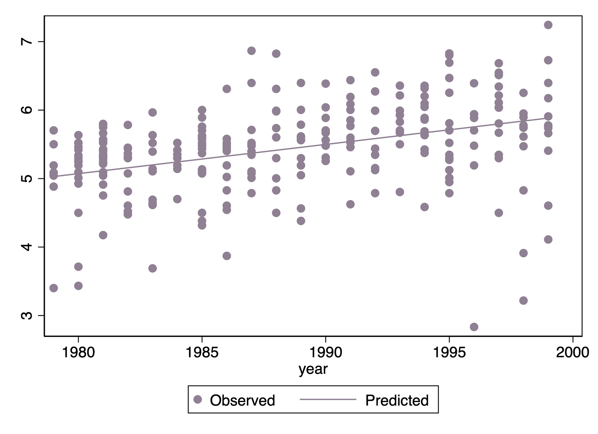
Figure 2: Observed and predicted log earnings for women aged 30 in Maine

The model estimates an annual change in wages of 4.26% (95% CI: 4.11 – 4.42%). It should be clear that we don't have a strong basis for saying there are no level changes in this data, and we cannot be sure that an arbitrarily chosen intervention group and and intervention period would be expected to have no significant effect. It should also be clear that this data is complex, and not suited for exploring a single specific issue in the technical details of a statistical model.

Now let us examine the issue of auto-correlation.

Is auto-correlation really the issue?

Before completing their simulations, the authors argue that there is strong auto-correlation in this data, and that this auto-correlation may drive the problem of under-estimation of standard errors. In section 2 they write:

The correlogram of the wage residuals is informative. We estimate first, second and third autocorrelation coefficients of the residuals from a regression of the logarithm of wages on state and year dummies (the relevant residuals since DD includes these dummies). The auto-correlation coefficients are obtained by a simple regression of the residuals on the corresponding lagged residuals. We are therefore imposing common auto-correlation parameters for all states. The estimated first order auto-correlation is 0.51, and is strongly significant.

This is a very confusing statement. The basic model they run here is the time/state fixed effects from equation (1), i.e. this model:

$$ Y_{ist}=A_s+B_t+\epsilon_{ist} \tag{2}$$

They then estimate the residuals, $ \hat{\epsilon}_{ist}$, and regress the residuals "on the corresponding lagged residuals". How did they do this? There are three indices in this data: i, s, t. Which index did they lag? For example, did they fix $i$ and $s$ and conduct this regression:

$$\epsilon_{ist}=\alpha+\beta \epsilon_{i,s,t-1}$$

or did they relabel their residuals with a single index covering all the observations, and then regress $ \epsilon_{j}$ on $\epsilon_{j-1}$? The problem here is that there is no sense of ordering over time in these data. For example, if they regressed data at time $t$ from state $s$ against data from time $t-1$ from state $s$, how did they choose which observation from time $t$ to pair with which observation from time $t-1$$? Regression relies on ordered pairs $(y_i,x_i)$, but in this case there is no information in the data set to justify any particular ordering. Furthermore, there are unmatched observations in each state-year. For example, there are 341 observations in 1980 in Maine, and 202 in 1979. How did they regress 341 observations on 202?

There is no time dependence in this data: no woman is observed in more than one year, something I checked with a few lines of code in the Stata script. So there is no concept of "lag" that can be applied to the residuals of this data. So I think the estimated auto-correlation they obtained from the regression they mention on page 7 is a complete fiction that tells us nothing about the actual auto-correlation in this data set. In fact, serial dependence in observations in different years that are not from the same individual does not make sense. It makes sense at an aggregate level – serial dependence of average logged wages over time within one state – but not at the individual level.

The next problem with the auto-correlation explanation is the values and their effect. For an auto-regression of lag 1 (an AR(1)), if we analyze the data on the assumption that it is IID (i.e. we do not adjust for auto-regression), the variance should be corrected by a factor of $\frac{1}{1-\phi^2}$, where $\phi$ is the magnitude of the auto-regression. In this case, with an estimated auto-regression (from those weird lagged residuals) of 0.5, we should expect the standard error to be deflated by about $\sqrt{4/3}$, or about 15%. It's unlikely that this level of deflation of the standard error is going to lead to a high level of false rejection of the null hypothesis, unless in thousands of simulations with the CPS data the null result was very close to significant in every case.

The level of auto-correlation needed to reduce the standard error of a coefficient in a multiple regression model to the point where it can massively inflate the risk of type 1 error is very large. The data show in Figure 1 is not consistent with such a level of auto-correlation, even if we could define auto-correlation clearly for this specific data set, which we can't.

There is another type of correlation in this data, which perhaps the authors meant to identify, which is the effect of clustering within states: since individuals within a state are more similar to each other than to individuals in other states, there is likely some small degree of correlation between observations within states that could be adjusted for using a cluster adjustment. This type of auto-correlation is usually associated with a design effect which is applied to inflate the variance, with the formula

$$DE=1+n_{s}\rho$$

where $DE$ is the multiplier applied to the variance, $n_s$ is the number of observations in state $s$, and $\rho$ is the intra-cluster correlation coefficient, a measure of the degree of similarity between observations within a state. Typically $\rho>0$, but usually $\rho$ decreases with the size of the state, since the larger the population from which we are sampling, the less likely observations are to be similar to each other. Typically $\rho$ is largest within families (when we can expect $n_s$ to be small, less than 10) and largest in diverse communities like countries, states or large counties. We don't usually see design effects bigger than 1.3-1.5, so it's unlikely that this is a major explanation for the way the TWFE models in this study reject null effects. While we should adjust for this, we should probably do this in a model that formally adjusts for the sampling design(2). In particular, this type of adjustment is applied at the level of the sampling unit, not at the level of the intervention, and only when the unit of analysis is different to the level at which sampling occurred. In the case of the CPS, sampling does not occur at the level of state, but in sampling areas within states, and clustering should be adjusted for the sampling areas, not the states. These effects aren't simple to calculate, but the CPS provides estimates of design effects for some elements of the sample (not ln wages, unfortunately), and they seem to be around 1.5 - 2, not enough to explain the effects that the authors have highlighted.

So, I don't think auto-correlation explains this.

How big are these effects anyway?

BDM2002 do not show the full results of their TWFE regression models, so we are left to guess at how serious the problem is from presentation only of the coefficient of the DiD term itself, which seems to be quite small. Here is their description of the magnitude of these effects, from page 12:

These excess rejection rates are stunning, but they might not be particularly problematic if the estimated “effects” of the placebo laws are economically insignificant. We examine the magnitudes of the statistically significant intervention effects in Table 3. Using the aggregate data, we perform 200 independent simulations of equation 5 for placebo laws defined such as in row 3 of Table 2. Table 3 reports the empirical distribution of the estimated effects β, when these effects are significant. Not surprisingly, this distribution appears quite symmetric: half of the false rejections are negative and half are positive. On average, the absolute value of the effects is roughly .02, which corresponds roughly to a 2 percent effect. Nearly 60% fall in the 1 to 2 % range. About 30% fall in the 2 to 3% range, and the remaining 10% are larger than 3%

So the problem appears to be that in general they estimate DiD effects that amount to a 1-3% increase in wages. Is this a big deal? We can test this quickly in Stata by making an arbitrary treatment assignment and treatment starting period. I do this in the Stata code, arbitrarily setting the first 25 states to be intervention states and starting the intervention at 1990. The DiD term and some time terms are shown in Figure 3.

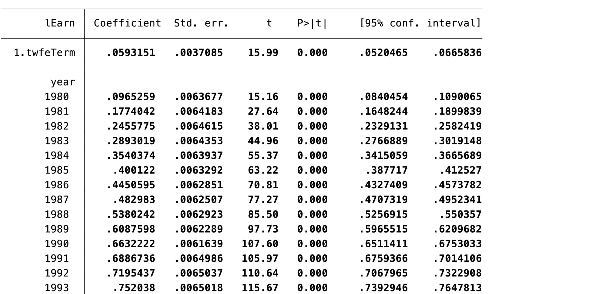
Figure 3: TWFE regression analysis of an arbitrary treatment scenario

The estimate of the DiD term is the coefficient of twfeTerm, which is 0.059 (95% CI: 0.052 - 0.067). That is about a 6% increase in the level of wages, after 1990. This is 2/3 of the change in wages from 1979 to 1980 (which was 0.097), and less than most annual changes occurring after that. It's essentially equivalent to 9 months of wages growth. That's not a very big effect! The authors argue that this should be interpreted as an elasticity in demand, and say 2% is big in this context, but I'm not convinced that this interpretation is valid. Do we interpret the 9.7% increase in wages from 1979 to 1980 as an indication that wage elasticity was 9.7% in 1979? I think we cannot interpret these estimates in that way.

Even if there is a particular interpretation of a term in a model that makes it seem physically unreasonable, we should still examine it in terms of what its basic mathematical properties are in the model. We can see that the standard error of the TWFE term is an order of magnitude smaller than the estimate. So even if the value of twfeTerm's coefficient was below 0.01, it would probably still be significant. This suggests that with a large number of observations like this, even very small numbers will be significant. This might be simply a problem of the size of the data set. None of these possibilities can be excluded because this simulation has been run with real data that has all the problems the real world brings with it. So let's re-examine how TWFE models work using a simulated data set.

Simulations

The R script bdm model.R defines a function called data.genBl() which randomly generates a data set suitable for testing the effectiveness of TWFE regression models. This function takes the following arguments:

txUnits, the number of treatment units; the total number of observational units will be twice this, with as many control units as treatment units
txPeriod, the total number of time steps in the data set, which must be 2 or more and even. The data generated by this function will have a control period equal to half of txPeriod, and a treatment period of the same length
dataRep, the number of repetitions of data in each treatment unit and time point. If dataRep=1 there will be a single observation in each treatment unit and time point, which is the classic framework.
baseMean, the mean of the first treatment unit in the first time point
varLim, a variable which controls the mean baseline differences between observational units. If varLim=0, all the units will have the same average at baseline. If varLim>0, the function will change the mean of each observational unit in the first time point by an amount drawn from a uniform distribution in the range $[-varLim,varLim]$. If varLim is large, the baseline differences between units will be quite large, drawn from a uniform distribution.
txEff, a variable that controls the effect of the intervention on the treatment units, all of which will be increased by a fixed amount txEff when the treatment period starts
spillEff, which determines how much the control group increases when the treatment period starts. This is the spillover effect, without which DiD models are unimportant. The true effect of the treatment on the treated units is txEff-spillEff
rndError, the standard deviation of the normally distributed residuals
plSlope, a slope term which, if it is not 0, causes all treatment units to have the same trend over time

If we run data.genBl() with 25 treatment units, txPeriod=20, about 300 repetitions, baseMean=5, varLim=0.2, txEff=spillEff=0, and plSlope=0.03 we can reproduce a situation vaguely similar to the simulation used by BDM, without any complicating non-linear effects or confounders. If we set the treatment and spill effects to 0, set varLim=0 and plSlope=0, we get a model where there is no baseline difference between units, no trend, and no treatment or spillover effects. In such a situation the TWFE model should produce a non-significant treatment estimate.

The two-way interaction regression model

Immediately after defining the function in the script file are a couple of lines where I generate different example data sets to investigate, and then two lines of code (lines 69 and 70) where I run two different DiD models. One (lm.true) is a classic two-way interaction model, and the other (lm.twfe) is the classic TWFE model. We have already seen the TWFE model. The classic two-way interaction model uses

$$y_{ist}=\alpha+\beta_1 x_{ist1}+\beta_2 x_{ist2}+\beta_3 x_{ist1}x_{ist2}+\epsilon_{ist}\tag{3}$$

where $X_1$ is an indicator variable for whether or not the i-th observation in the s-th group at the t-th time point is in the treatment or control group,

$X_{ist1}=1$ if the observation is in the treatment group
$X_{ist1}=0$ if the observation is in the control group

Since this indicates group membership it is 0 or 1 across the entire series of time points for each individual. The coefficient of $X_1$, $ \beta_1$, measures the average difference between treatment and control groups at baseline, and its value will depend on the distribution of average values at baseline. Since these are random, it's not a particularly important value.

$X_2$ is a variable that indicates whether an individual is in the treatment or control period,

$X_{ist2}=1$ if the observation is in the treatment period
$X_{ist2}=0$ if the observation is in the control period

Note that $X_2$ changes at the same time for every individual observation in the data set. The coefficient of $X_2$, $\beta_2$, measures the change in the control group after the intervention starts. If $spillEff$ is not 0, we should expect $\hat{\beta_2}\approx spillEff$, or at least that its confidence interval includes the value of $spillEff$.

The interaction term $\beta_3$ measures the additional effect of the intervention in the intervention group. It is mechanically equivalent to $\beta$ in equation (1), and for our simulated data we should expect $\hat{\beta}_3 \approx txEff-spillEff$.

The big difference between the classic two-way interaction model and the TWFE model is that the latter attempts to estimate the baseline differences between intervention groups and to calculate the specific deviation of each time point from the long-term average. We don't care about these numbers, and the classic two-way interaction model doesn't waste time on them. This will mean that as the value of $varLim$ increases above 0 the standard deviation of the residuals in the classic two way interaction model will increase, while in the TWFE model it will remain approximately equal to $rndError$.

This leads me to a suspicion that the standard error of the treatment effect in the classic two-way interaction model will depend on the baseline differences in the treatment units, while the standard error of the TWFE model will depend on the sample size only. Before we build our simulation study of false rejection, we will test this.

Simulation results

We run three simulation models, numbered as such:

Comparison of standard error of treatment effects for different degrees of baseline variation between treatment units
Test of probability of falsely rejecting the null for different sample sizes and baseline structural effects
A brief and not comprehensive power assessment

We use the data.genBl() function for all of these tasks, which are set out in the R script in three separate sections.

Simulation 1: Effect of baseline structure

Before testing the rejection rate of the basic TWFE model I wanted to confirm that the standard error of the TWFE model does not depend on the baseline structure of the difference between the treatment units. To do this I simulated data with no treatment effect, no spillover effect, no slope, 25 treatment units, 25 control units and 20 time points (10 for control period and 10 for intervention period). I varied the limits of the uniform distribution that drives the baseline separation of the observational units from 0 (all of them with the same baseline mean) to 10 (each baseline mean modified by a value uniformly distributed between -10 and 10) in steps of 0.1.

At each of these sets of parameters I ran 100 simulations with 10 individuals per observational unit and random residual error (all with SD of 1), applied the classical two-way interaction model and the TWFE model, and calculated the standard error of the estimate of the treatment effect. I summarized this in a table with the mean SE of the 100 runs and its interquartile range.

In this simulation, with no differences between baseline treatment units (varLim=0), the standard error of the treatment estimate from both the classic two-way interaction model and the TWFE model was about 0.04. As the spacing between treatment units increased the standard error of the two-way interaction model increased, but it remained the same at 0.04 for the TWFE model. Some summary figures from four representative sets of simulations are shown in Table 1 (I don't show IQRs).

Range of baseline values	Two-way interaction model SE	TWFE model SE
0	0.040	0.040
-0.5 – 0.5	0.041	0.040
-3.0 – 3.0	0.078	0.040
-5.0 – 5.0	0.118	0.040
-7.5 – 7.5	0.173	0.040
-10.0 – 10.0	0.450	0.040

Table 1: Invariance of standard error to baseline conditions in the TWFE model

By way of reference, the baseline mean used in generating this data was 20, so in the final simulation the observational units have baseline means varying between 10 and 30, with no structural difference between intervention and control groups.

This should make it clear that regardless of the structure of the differences between baseline effects, the standard error of the TWFE model seems to depend only on the sample size. This makes sense, since the model is capable of modeling every part of the structure (the arbitrary differences between time points and the arbitrary differences between observational units at baseline), leaving only the randomness of the data. In contrast, as structural differences between the baseline means increase, the two-way interaction model only estimates the average difference between control and intervention groups, and all other differences are absorbed into the residual error, which will lead to increases in standard error.

This suggests that as the sample size grows, the TWFE model is highly vulnerable to even very small differences in trend between intervention and control groups, which might be too small to identify with visual inspection. This should give a clue as to why the simulation in BDM 2002 found a significant effect of treatment - with 300,000 observations and 25 treatment groups, even a tiny amount of curvature, or tiny differences in trend between intervention and control groups, will register as significant.

But what happens if we remove all those unknown factors of real data, and model a simple data set where there is no curvature, no covariates, and no differences in trend at all? Would we reject the null very frequently then?

Simulation 2: Probability of falsely rejecting the null

To test whether the TWFE model falsely rejects the null more often than we might expect from chance I simulated data with a baseline mean of 24 and a residual error of 1, with a number of replicates for each observational unit of $1, 2, 4, 8, \ldots, 512$. I set the study period to be 20 time points (10 before the intervention, 10 after), with 25 treatment and 25 control units. I ran it with no random baseline variation between observational units, and then increased this so that varLim ran from 2 to 10 in steps of 2. I then applied the TWFE and two-way interaction models to the data, and recorded whether the treatment effect was significant for each model.

At each combination of observational units and variation of baseline means I ran 100 simulations and calculated the proportion of simulations that were significant. It should be noted that, because I'm a poor programmer, this simulation takes quite a while.

The results were completely different to the results of the BDM 2002 paper. Depending on the number of observations in each observational unit and the range of baseline means, rejection rates for the TWFE model ranged from 0% to 14%. Rejection rates for the classical two-way interaction model ranged from 2-7% when there was no difference between baseline means, and were 0% for all other scenarios.

Table 2 shows some illustrative combinations of baseline differences and sample sizes (the full results can be obtained by running the code in the R script). I hope this table shows that, in the absence of poorly managed confounders and unexpected trends and curvature, the TWFE model handles null scenarios perfectly fine, with rejection rates broadly consistent with a 5% significance level.

Treatment difference	Individuals per observational unit	Two-way interaction rejection rate	TWFE rejection rate
0	1	0.02	0.02
0	16	0.04	0.04
2	1	0.00	0.05
2	4	0.00	0.00
2	128	0.01	0.05
4	1	0.00	0.06
4	16	0.00	0.07
6	1	0.00	0.04
6	64	0.00	0.14
8	1	0.00	0.02
8	512	0.00	0.06
10	1	0.00	0.07
10	256	0.00	0.07

Table 2: Rejection rates from a properly-specified null model

So, the TWFE model does not need to be adjusted for clustering in its basic form. Unless we have a good reason for thinking that there are strong clustering effects within the observational units (not over time), there is no reason to trouble ourselves with this problem. If the TWFE is overly generous in rejections, it is much more likely to be due to some small differences between intervention and control groups than have been accounted for in the model, or non-linearity or a missed trend effect. We will return to this when we apply a more advanced form of the two-way interaction model to the CPS data.

Before we do though, we note that the two-way interaction model has a 0% rejection rate in most cases, which suggests it might be preferable to the TWFE model on this issue. However, we have seen that the standard error of the DiD term increases in the two-way interaction model as baseline structure changes, so could that low rejection rate arise because the model also has low power, and is unable to identify small effects? Let's briefly investigate that.

Simulation 3: Power assessment

The third simulation in the R script loops through different possible intervention effects and assesses the effectiveness of the TWFE and classical two-way interaction model at testing these effects. It runs simulations of the data using the dataGenBl() function with a small treatment effect of 0.5, 1 or 2, for 25 treatment units and 20 time points, with no spillover effect in the control group and either 1, 2, 4, 8 or 16 individuals per observational unit. For all simulations there is no slope, a residual standard deviation of 1, and the baseline mean of each observational unit is allowed to vary uniformly between 14 and 34.

In this scenario a treatment effect of 0.5 is equivalent to an average $\frac{0.5}{24}\approx 0.02$ increase in the mean, i.e. a 2% increase. It's not meaningful in a policy sense! But we still want to know whether either of our modeling strategies is able to identify this. Table 3 shows some estimates of the mean bias of the models and the probability that they reject the null hypothesis, for selected combinations of the size of the treatment effect and the number of individuals per observational unit. Recall that in these simple settings the TWFE and two-way interaction models produce the same coefficient estimates, and differ only in the standard error of those estimates, so only one bias estimate is reported.

Treatment effect	Individuals per unit	Mean bias	Null rejection, classical two-way	Null rejection, TWFE
0.5	1	0.001	0%	99%
0.5	2	0.012	0%	100%
0.5	4	-0.015	1.0%	100%
0.5	8	-0.002	54.0%	100%
0.5	16	0.005	100%	100%
1.0	1	-0.027	0%	100%
1.0	2	0.009	57.0%	100%
1.0	4	-0.028	100%	100%
2.0	1	-0.005	100%	100%

Table 3: Probability of rejecting the null and mean bias of estimated treatment effects in different modeling scenarios

By playing with the vectors of treatment effects and replicates you can generate different scenarios in the simulation. You could also try extending it to allow non-zero slopes, different levels of random error, or different magnitudes of baseline error, but I hope it is clear from this simulation that the TWFE model has very high precision, and as a consequence of its tendency to pick out even the smallest random variations between treatment units or time points as structure rather than error it is able to correctly identify even very small effects with a high degree of success, without necessarily sacrificing confidence in the case of null effects.

If you have sufficient observations, time points or treatment units, and you want to be sure that you have no risk of falsely rejecting a null scenario, the two-way classical interaction model is better, but if your sample size is small and/or your likely effect sizes are very small, TWFE is better. But in neither case do you need to adjust for clustered variances to ensure that you don't falsely reject the null.

A better model for the CPS data

(Reader note: This section involves some fairly nasty linear modeling and doesn' prove much, so feel free to skip it if you don't want your eyes to bleed).

Before we conclude this discussion, let us consider a more sophisticated application of the two-way interaction model to the original CPS data that was used in the example. We will now generate a set of variables measuring 5-year age groups,

$ Z_{istj}=1$ if the observation is in the j-th age group
$ Z_{istj}=0$ otherwise

where here $j\in[1,\ldots,6]$, with $j=1$ corresponding to 25-29 year olds, $j=2$ corresponding to 30-34 year olds, and so on up to 50 year olds (the final age group is only one year in width because of the strange age limitation enforced on the data by BDM). We then build the following model:

$$y_{istj}=\alpha+\beta_1 x_{ist1}+\beta_2 x_{ist2}+\beta_3 x_{ist3}+\sum_{j=2}^{6}\gamma_j z_{istj}+\sum_{j=7}^{11}\gamma_j z_{ist,j-5}x_{ist1}+\beta_4 x_{ist2} x_{ist1}+\sum_{j=12}^{16}\gamma_j z_{ist,j-10}x_{ist2}+\beta_5 x_{ist2}x_{ist3}+\epsilon_{ist}$$

This looks horribly complex(3), but only because of the presence of the age dummy variables. Here we define the following variables in addition to the age group dummy variables:

$X_1$ is time, shifted so that it is 0 in the year 1990
$X_2$ is treatment group, defined as in the two-way interaction model introduced above
$X_3$ is treatment period, defined as in the two-way interaction model introduced above

So, when $X_2=0$ an observation is in the control group, and when $X_2=1$ it is in the treatment group. When $X_3=0$ the observation is in the pre-treatment period, and when $X_3=1$ it is in the post-treatment period. $X_2$ is fixed at baseline for all observations, while $X_3$ changes at the point of intervention for all observations (even those in the control group). Then the coefficient $\beta_5$ defines the DiD effect.
The other, horribly complex terms are interpreted as either age effects, age-time interactions, age-treatment interactions, or treatment-time interactions. For example, the term
$$\sum_{j=2}^{6}\gamma_j z_{istj}$$
measures age effects: for any given observation, $z_{istj}=1$ for precisely one value of $j$, and 0 for the rest, and this one non-zero term is the effect of age group $j$ on the response. We start at $j=2$ in order to set age group 1 as the reference level, i.e. to have 25-29 year olds as the reference age group.
The term
$$\sum_{j=7}^{11}\gamma_j z_{ist,j-5}x_{ist1}$$

measures age group time interactions. For example when $j=7$, we have $z_{ist,j-5}=z_{ist2}$, which is 0 if the $i$-th individual in the $s$-th treatment group at the $t$-th time point is not aged 30-34, and 1 if they are in this age group. If the person is in this age group then the expression simplifies to $\gamma_7 x_{ist1}$, which is a modification to the time trend in age group 2. For each individual this set of sums will pick out a single term that modifies the trend in the corresponding age group (age group 1 remains unmodified and its slope can be estimated directly by $\beta_1$). So, for example, the estimated slope in age group 2 (30-34 year olds) will be $\beta_1+\gamma_7$. This enables us to have different trends in wages by age group, which is a completely reasonable assumption for modern wage data!
The next term, $\beta_4 x_{ist2} x_{ist1}$, allows for a different trend in treatment and control groups. If the subject is in the control group then $x_{ist2}=0$ and this term disappears; if they are in the treatment group we have $x_{ist2}=1$ and this term becomes $\beta_4 x_{ist1}$, which is a modification to the trend term that applies in the treatment group only. If the person is aged 25-29, the slope will be $\beta_1+\beta_4$; if they are aged 30-34 it will become $\beta_1+\beta_4+\gamma_7$, and so on. With this construction people in the treatment and control groups are able to have different slopes.
The final beastly term measures an age group/treatment interaction:

$$\sum_{j=12}^{16}\gamma_j z_{ist,j-10}x_{ist2}$$

This allows the difference between treatment and control groups to differ by age. For example, when $j=12$ we have the term $\gamma_{12} z_{ist,j-10}x_{ist2}=\gamma_{12} z_{ist2}x_{ist2}$ which will be 0 if the observation is not in age group 30-34, and will take the value $\gamma_{12}x_{ist2}$ if they are in age group 30-34. Further, if they are in the control group we have $x_{ist2}=0$, so this term disappears, but if they are in the treatment group $x_{ist2}=1$ and this term becomes $\gamma_{12}$. So this sum picks out a single coefficient $\gamma_{j},j\in 12,\ldots,16$, such that the difference between treatment and control groups will be modified by $\gamma_j$ when the subject is in age group $j-10$. Thus, for example, if someone is in age group 25-29 all the terms will be 0 and the difference between treatment and control groups is given by $\beta_2$; but if they are aged 30-34 the difference between the treatment and control groups is given by $\beta_2+\gamma_{12}$.
This model simultaneously allows us to model:

Differences in baseline salary by age group ($\gamma_{2},\ldots,\gamma_6$);
The difference between treatment and control groups ($\beta_2$),
Where this difference varies by age group ($\gamma_{12}, \ldots, \gamma_{16}$);
A time trend ($\beta_1$)
Where the time trend differs by age group ($\gamma_{7},\ldots,\gamma_{11}$);
And the time trend differs between intervention and control groups ($\beta_4$);
Where there is a potential change in the control group when the intervention happens ($\beta_3$)
Where the additional change in the intervention group can be estimated ($\beta_5$)

In this model the estimate of the DiD effect, $\beta_5$, is adjusted for the possibility of non-parallel trends in the intervention and control groups, non-parallel trends in the different age groups, and different baseline averages between age groups and between treatment and control groups. We could go further with three-way or four-way interactions to model changes in trend at the time of the intervention, changes in the relationship between wages and age group at the time of the intervention, and so on. But since we know the intervention isn't real, why bother?
The final section of the Stata code fits this model for an imaginary intervention starting in 1990. Note that the time variable is shifted so that 1990 is 0, enabling the constant to be estimated as the average value in a 25-29 year old in the control group in 1990(4). The results of the model are shown in Figure 4.

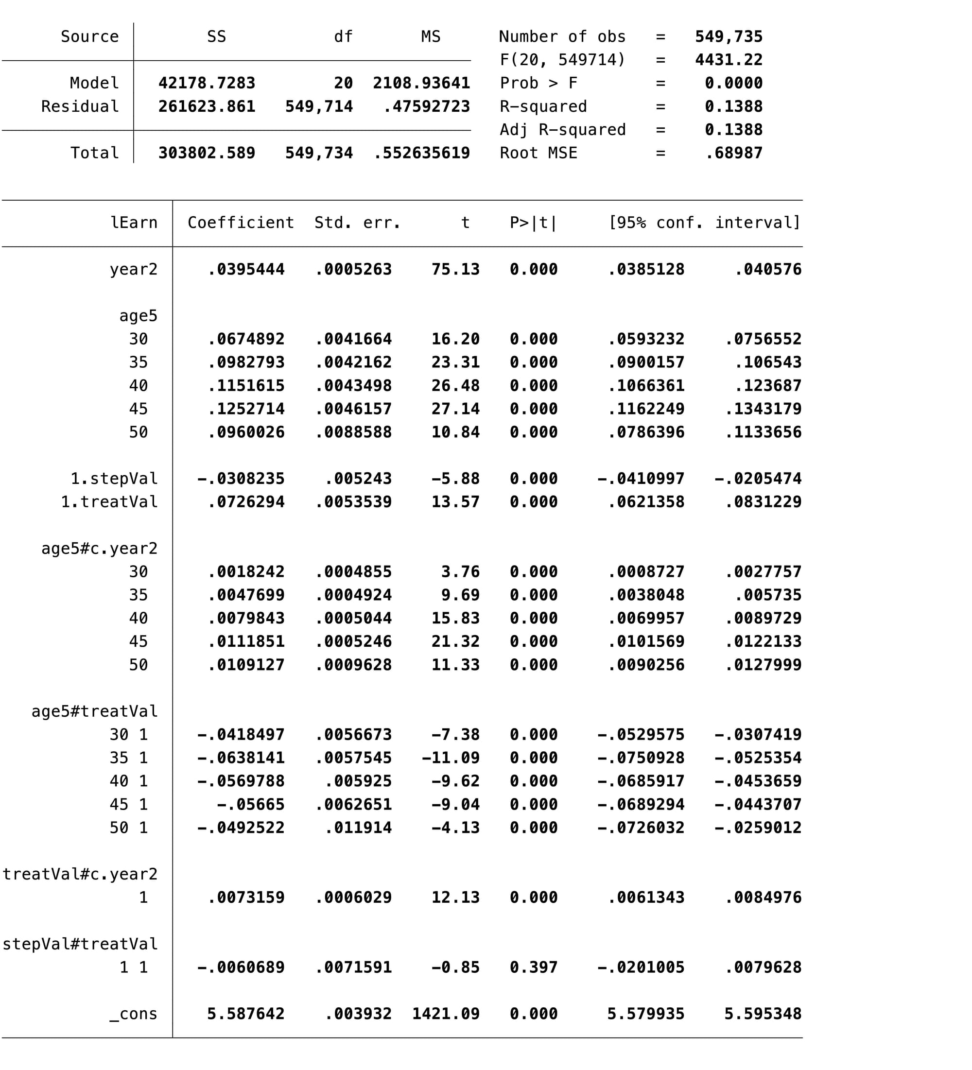
Figure 4: Results of classical interaction model of the CPS data from BDM 2002

The final term before the constant, stepVal#treatVal, is the DiD effect, and look! It's very very very small and completely non-significant. But note what is significant:

Highly significant differences in salary by age
Highly significant time trend
Significant, but very small downward step at the time of the intervention, common to treatment and control groups
Significant difference between treatment and control groups at baseline
Highly significant differences in trend by age group (the age5#c.year2 terms)
Highly significant modification of the difference in wage between treatment and control groups, depending on age (the age5#treatVal terms), with the largest difference between treatment and control groups occurring in the youngest people
A small but significant difference in trend between treatment and control groups (the treatVal#c.year2 term)

Of course there are many other ways we could model the CPS data, and there are model-building strategies to sort between them, but the key indication from this model is that you can't simply throw an arbitrary model at a simulated intervention with the CPS data and conclude that it means classical regression methods don't work. The conclusions we draw from this CPS data are subject to too many possible model-based confusions, what Gelman refers to as the "garden of forked paths".

This data is simply not very useful data for simulation, and there is a strong lesson here for people planning to use simulation to explore the potential of models: don't use real world data where you don't know what the truth is, because you will never be able to separate the flaws in the model from the real but unknown patterns in the data.

Discussion

The original BDM2002 paper used a pseudo-simulation of real-world CPS data to argue that two way fixed effect (TWFE) models are highly likely to falsely reject the null. They ran a series of models in which they assigned a random 50% of states to an intervention group and started the intervention at a random time point, then estimated the DiD effect using a TWFE model with adjustment for a complex function of age and a term for education. About 60% of the time the TWFE model found a significant DiD term even though they assume no intervention occurred in this time series.

After establishing that this high rate of false positives the authors argued that this is likely due to auto-correlation in the data. They identified this auto-correlation by regressing residuals from a simple fixed-effects model on the "lagged" residuals from this model, and argued based on this "correlogram" that there is significant auto-correlation in the residuals, probably induced by the use of a TWFE term, and that this auto-correlation explains the high rejection rate. They then presented four solutions to this problem, which I have not described here but which mostly seem to me to be disastrous. However, none of these solutions are necessary because the problem they identified is not real, and we don't need to worry about it.

I showed that this problem is not real by first addressing their simulation study, then investigating their methods for estimating serial dependence, and then examining the properties of the TWFE model in a little more detail using more reliable data that I simulated myself. The tools I used to do this in R and Stata can be found on my Github.

First, in addressing the simulation, I noted that the CPS data they used for their simulation has a rich and complex set of relationships that we do not fully understand. I argued it is possible that there are small differences in trends between treatment and control groups, and/or curvature in the data that is not fully captured in the model, and/or differences in patterns of data by age and time period. If there is any part of the underlying "truth" of this data that has not been captured in BDM's regression models, then the DiD term could capture some element of that truth and reject the null hypothesis. In short, we don't know if the hypothesis shouldn't be rejected. I also pointed out that the effect size of the DiD estimate is much smaller than the annual changes in the data that can be estimated from the time fixed effects, and therefore could just reflect some residual error. I argue we cannot draw any conclusion from this data.

I then investigated the "auto-correlation" the authors presented as the cause of this false rejection rate. I argued that their estimation of auto-correlation is statistically meaningless, at least to the extent we can understand it from their presentation of their methods. It is not possible to estimate auto-correlation from their CPS data, since its structure is inconsistent with the concept. I also used some basic expressions for variance inflation in the presence of auto-regression to argue that the effect they identified would not be large enough to cause the high rate of rejection they found in their simulations. I identified other possible inflation of variance that could occur due to breaches of the IID assumptions of OLS regression, but suggested that these were not properly adjusted for in the BDM2002 paper, and everything we know about their effects suggests they would not be large enough to drive a large false positive rate. I suggested instead that a better set of simulations is necessary to explore this phenomenon.

I then ran these simulations, generating data with a known structure, and showed that the TWFE model actually has rates of type 1 error that are not very different from those we would expect from random chance. I compared it with another regression framework, classical two-way interaction, and suggested it has slightly better power than this framework but a higher risk of type 1 error. I think that there is a possibility that in a very large sample like the CPS sample used in this paper it is possible for a TWFE model to have a higher risk of type 1 error because of the way it spuriously identifies random error as structure (as shown by its estimate of significant time fixed effects in a model with no significant time trend). This is also the reason it has high power when a classical regression model would have very low power.

Finally, I constructed a more sophisticated model for the CPS data which accounts more carefully for time trends and variation between age groups and treatment and control groups, and showed that it is possible with this model to generate a non-significant result. I did not bother simulating this as they did in the BDM2002 paper, because we cannot draw any conclusions from a simulation using data with an unknown data generating process.

Conclusion

You don't need to cluster variance in your TWFE models, because the claim from BDM2002 that these models have overly high rates of rejecting the null does not hold up under proper investigation of properly-controlled simulated data. Although you should adjust for the clustering of data, you should do this in a formal way that properly accounts for the probability of sampling and the survey design, which BDM2002 did not do, and which to the best of my knowledge econometricians never do.

Although there are problems with TWFE regression designs, high rates of rejecting the null are not, in general, one of them. If you cluster your variance estimates you just risk reducing power to no purpose, and there is no formal statistical reasoning that supports arbitrary clustering of variances. Don't do it!

Footnotes

Actually they do this in a slightly backwards order, first showing the auto-correlation problem, then doing the simulation
Incidentally, this CPS data does have a sampling design, and there is no evidence that the authors of this paper properly accounted for it when they ran the regression models; they should have used sampling weights and a proper svyset command before analyzing this data, which in itself might have solved their problem!
I intend to follow this blog post with a similarly exhausting post on how to work with interaction terms, a massively under-rated tool in statistical analysis of policy interventions!
We need to be very careful with the position of the intercept when we do this sort of modeling, because if it is set to the wrong value all of the estimates of differences in level will measure strange counterfactuals. If you want to know what the difference in female salaries would have been by age in the year that Jesus was born, leave your time variable so that it starts at 1990!